Filter and CCD Characteristics

Here is described a way to combine information about the filter bandpass specification (transmission vs wavelength) with information about the CCD detector response (quantum efficiency vs wavelength). Doing this helps to understand how to time or equalize exposures, and how to compensate for differences in filters and CCD sensitivities, or how to plan for special observing. The computations below are pretty good approximations, but they are only approximations.

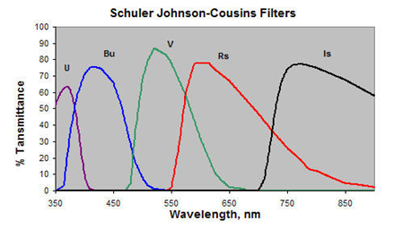
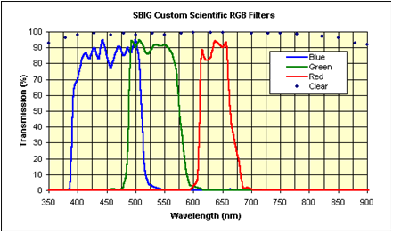
The Filters

Here are two graphics illustrating the filter bandpasses for Schuler UBVRI and SBIG RGB filters. This information comes from data published by the manufacturers, and it should be provided by the manufacturer for any filter. On the left are the traces for the Schuler U, Bu, V, Rs and Is filters. They show the amount of energy passed through the filter at various wavelengths. These are very similar to the traditional Johnson UBVRI filters. A similar figure for the SBIG RGB and Clear filters is on the right.

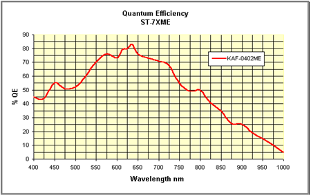
The CCD

The third graphic, below, shows the quantum efficiency of one particular detector, the Kodak KAF-0402ME. This graphic illustrates how much of the light at a given wavelength is converted to an electric current. Or notionally more simply, the percentage of incident photons are converted to electrons at a given wavelength.

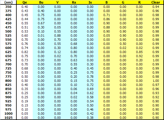
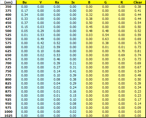
Tabular Data

This graphic illustrates in tabular form what the figures above show graphically. The first column is the wavelength in nanometers. The remaining columns list the response of the CCD(Qe) (second column) or transmission of the filters (Bu...Clear) as estimated from the graphics.

TABLE I.

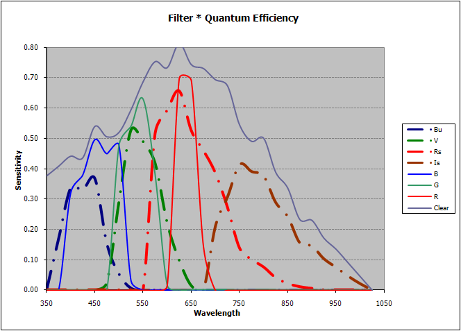
Combining the Data

How these data are combined is what gives us the interesting insight into what should be expected out of a filter-CCD system. Multiplying each value in the second column from each row of the table above (Qe) across the row results in the table below. This provides an estimate of the combined response function of the filter-CCD system as a whole, as a function of wavelength. These results are also shown in the graphic below the table.

TABLE II.

FIGURE I.

A look at this graphic reveals several interesting observations:

The RGB filters (narrow red, green and blue lines) yield better color reproduction that the Schuler Rs, V, Bu filters (thick dot-dash lines) because the RGB filters are "sharper," with less or little crossover of the edges of the filter. They're made this way on purpose so as to isolate specific parts of the visible spectrum of light.
As seen from the graphic, the Schuler V filter and the traditional G filter will both collect about the same total energy. This is the sum total of all the light coming through the filter across its total bandwidth. Another way to say it is that the area under these two green curves is about the same. This is not true for either the red or the blue filters.
The exposure times needed to image through any of these filters depends naturally on the size of the "window" each of these filters opens. Thus, for the same exposure time, images taken through the Schuler Rs filter will reach about 1 magnitude "deeper" than images taken through a "Red" because the Schuler "window" is about 2½ times bigger than the R filter is.

Integrated Flux

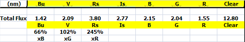
Using the table above in "Combining the Data" and summing down each column gives the following table. In this table the row called "Total Flux" compares in a relative way the light gathering power of this particular filter-CCD combination. So for this system, disregarding the Clear filter which will always take in more light, the Rs filter has the biggest "window." Taking the ratio of Rs to R gives 3.80/1.55 = 2.45, which is approximately equivalent to one magnitude difference, as mentioned above. Thus, imaging throught the Rs filter will reach one magnitude fainter than imaging through the R filter, other things being equal (which they're not!).

When imaging through RGB filters, where the ratios of fluxes are B=2.15 :: G=2.04 :: R=1.55, one can reach the same depth with the same exposure in B and G filters, but must increase the exposure time by an amount equal to ~2.1/1.55, or 1.35x.

TABLE III.

  This is not the end, however.

The Effect of Star Colors

  All of the above has not factored in how the Integrated Flux changes depending on the color (spectral type, surface temperature) of the stars in an image. What's been assumed up to now is uniform white light across the spectrum. This is, of course, not true for real objects. A star's or object's color will alter the filter-CCD response by introducing another weighting factor. The result is that the values in the table in the section Combining the Data will be modified differently for each object having a different surface temperature (color, spectral type). This will lead to a different Total Flux for each type of star.

  Here's an animation of the filter graphic above, for which the spectral effect of O, B, A, F, G, K & M, with a surface temperatures of ranging from 40,000°C (O-type stars) to 3,000°C (M-type stars), has been included. The seven-frame animation shows the relative strengths of the filters normalized to the peak of the CLEAR filter.

FIGURE II.